What is FVM?

FVM is a Formal Verification Methodology for digital microelectronics. Its main objective is to lower the adoption barriers for Formal Verification for the European Space Sector, although it can be used in many other contexts where digital design and/or verification is performed, such as teaching, research, avionics, automotive, etc.

Its development is funded by the European Space Agency, through its Open Space Innovation Program, specifically the activity “Lowering the adoption barriers for Formal Verification of ASIC and FPGA designs in the space sector”. The activity is being implemented by Universidad de Sevilla (Spain), through its affiliated Technology Centre AICIA (Asociación de Investicación y Cooperación Industrial de Andalucía).

The FVM is available under the permissive free/open-source license Apache License 2.0

Components

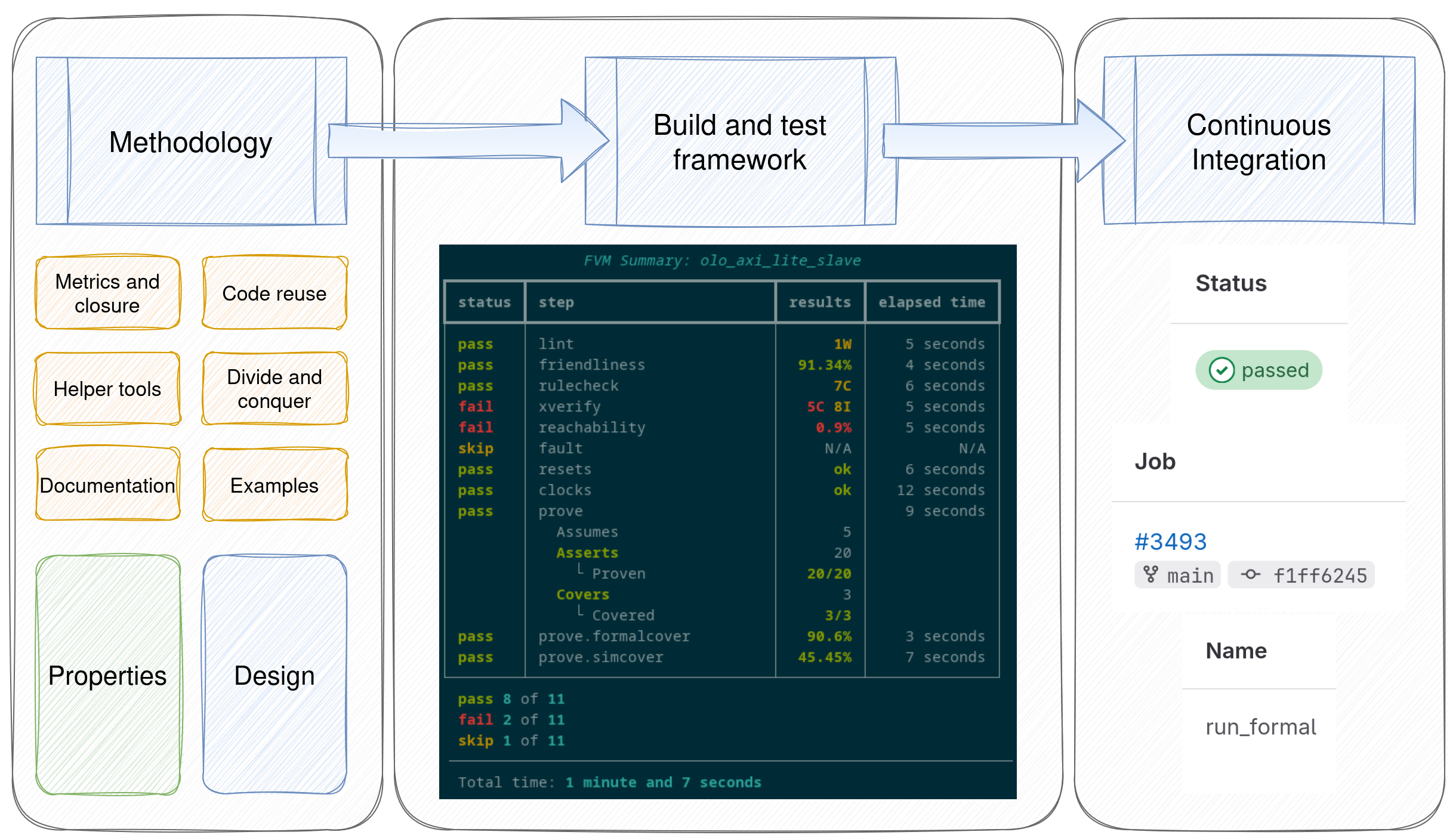
The different parts of the FVM are:

• A defined methodology, with detailed steps.

• Helper tools that reduce the learning curve and effort required to write the formal properties

• A build and test framework that acts as an abstraction layer to interface with the software tools, generates XML files for Continuous Integration systems, and creates reports.

• A repository of examples, in increasing order of difficulty, that serve to introduce the concepts of the FVM gradually, with self-sustaining examples that can be studied and understood incrementally.

• Documentation and training materials to help new users understand both formal verification in general, and the FVM. You are reading those :)

A graphical summary of the FVM can be found below:

The methodology steps

As FVM is a methodology, it starts by defining a number of steps to perform:

The steps can be organized as follows:

• Leverage any available automated tools

• Create properties for the design under verification, leveraging the provided helper tools

• Run a model checking / property checking tool to prove or disprove the defined properties

• Generate reports and coverage metrics, including simulation metrics for traces generated in the previous step

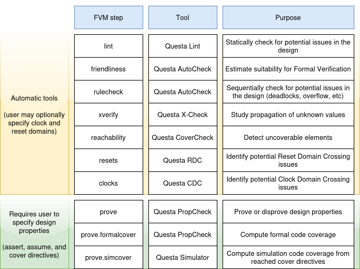
The diagram below expands the list, since there are many automated tools available:

The build and test framework

The FVM framework acts as an abstraction layer that interfaces with the formal tools. Each formal tool may require different configurations and commands, and FVM manages that for you, while also providing sensible defaults for tool options.

The user just writes a simple formal.py script like the following one:

from fvm import FvmFramework

fvm = FvmFramework()
fvm.add_vhdl_source("examples/counter/counter.vhd")
fvm.add_psl_source("examples/counter/counter_properties.psl", flavor="vhdl")
fvm.set_toplevel("counter")
fvm.run()

When running the script (python3 formal.py), the framework automatically calls the different formal tools, collects the relevant metrics, and generates the reports.

Supported toolchains

Currently, just the Questa Formal Tools (and Questa Simulator, for the simcover step) are supported

The following table relates each FVM step with the relevant Questa tool

FVM and the Questa toolchain

FVM step	Questa tool
lint	Lint
friendliness	AutoCheck
ruleCheck	AutoCheck
xverify	X-Check
reachability	CoverCheck
resets	RDC
clocks	CDC
prove	PropCheck
prove.formalcover	PropCheck
prove.simcover	QuestaSim

drom2psl

drom2psl is a package provided with FVM that aims to reduce the learning curve and necessary effort to define formal properties.

From a Wavedrom .json file, sequences are extracted, even with parameters.

For example, from the following .json file:

{
head: {text: 'wb_classic_read(addr, data)',
    tick:  0,
    every: 1,
    },
foot: {text: 'Wishbone read, classic mode',
    },
signal: [
    {name: 'clk',   wave: 'p|.|'},
  ['Master',
    {name: 'adr', wave: 'x3.x', data: 'addr', type: 'std_ulogic_vector(31 downto 0)'},
    {name: 'dat', wave: 'x...'},
    {name: 'cyc', wave: '01.0'},
    {name: 'stb', wave: '01.0'},
    {name: 'sel', wave: 'x...'},
    {name: 'we',  wave: 'x0.x'}
  ],
{},
  ['Slave',
    {name: 'dat', wave: 'x.3x', data: 'data', type: 'std_ulogic_vector(31 downto 0)'},
    {name: 'ack', wave: '0.10'},
    {name: 'err', wave: '0...'}
  ],
],
}

Which corresponds to the following waveform diagram:

The following PSL file is generated:

vunit wishbone_classic_read {

  sequence wishbone_classic_read_Master (
    hdltype std_ulogic_vector(31 downto 0) addr
  ) is {
    ((Master.cyc = '0') and (Master.stb = '0'))[*1]  -- 1 cycle;
    ((Master.adr = addr) and (Master.cyc = '1') and (Master.stb = '1') and (Master.we = '0'))[+]  -- 1 or more cycles;
    ((Master.cyc = '0') and (Master.stb = '0'))[*]  -- 0 or more cycles
  };

  sequence wishbone_classic_read_Slave (
    hdltype std_ulogic_vector(31 downto 0) data
  ) is {
    ((Slave.ack = '0') and (Slave.err = '0'))[+]  -- 1 or more cycles;
    ((Slave.dat = data) and (Slave.ack = '1') and (Slave.err = '0'))[*1]  -- 1 cycle;
    ((Slave.ack = '0') and (Slave.err = '0'))[*]  -- 0 or more cycles
  };

}

Repository of examples

To ease the learning curve, examples on how to formally verify a number of designs of increasing complexity are provided. These designs are ordered so the FVM can be learned by working through them. See Repository of Examples for more information.